Introduction

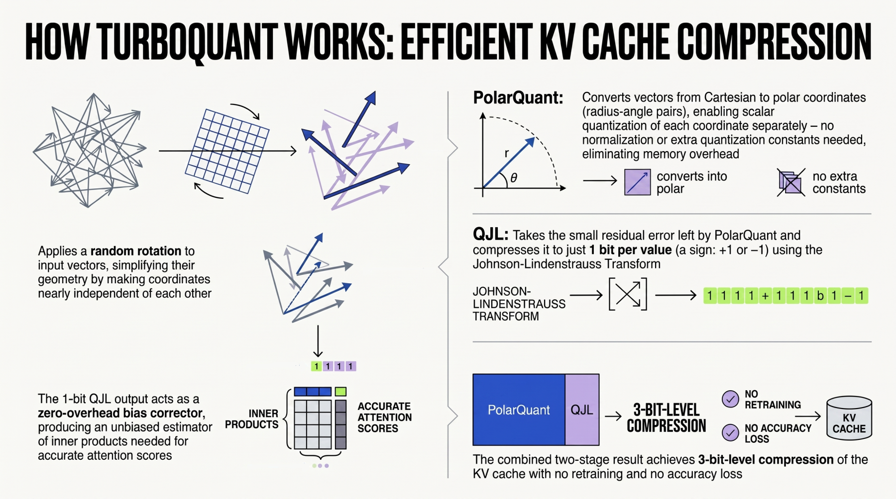
Large language models (LLMs) and retrieval-augmented generation (RAG) systems rely heavily on efficient key-value (KV) cache management. The KV cache stores intermediate attention states, enabling faster inference but consuming enormous memory—often becoming a bottleneck. Google's TurboQuant offers a novel algorithmic suite and library that applies advanced quantization and compression techniques specifically to LLMs and vector search engines. This guide walks you through compressing your KV cache using TurboQuant, step by step, so you can reduce memory footprint without sacrificing accuracy.

What You Need

• Hardware: A machine with a CUDA‑capable GPU (NVIDIA V100, A100, H100, or similar) with at least 16 GB VRAM for initial testing.
• Software prerequisites:
  • Python 3.8 or higher
  • PyTorch 2.0+ (with CUDA support)
  • Hugging Face Transformers library
  • Git (to clone the TurboQuant repository)
  • A C++ compiler (GCC or Clang) for compiling optional extensions
• Model & data: An LLM you wish to compress (e.g., Llama 2, Mistral, or Gemma) and a representative calibration dataset (e.g., a few hundred samples from WikiText or your domain).
• TurboQuant library: Clone from Google's official repository (replace with actual URL if known) and install dependencies with pip install -r requirements.txt.

Step‑by‑Step Guide

1. Step 1: Prepare Your Environment

   Set up a virtual environment to keep dependencies isolated. Use python -m venv turboquant_env and activate it. Install PyTorch with the appropriate CUDA version. Then install TurboQuant by cloning the repo and running pip install -e . from within the repository root. Verify the installation by importing turboquant in Python without errors.

2. Step 2: Load Your LLM

   Use Hugging Face's AutoModelForCausalLM to load the target model in half‑precision (fp16) to save VRAM initially. Example:
   from transformers import AutoModelForCausalLM, AutoTokenizer
model = AutoModelForCausalLM.from_pretrained('meta-llama/Llama-2-7b-hf', torch_dtype=torch.float16, device_map='auto')
tokenizer = AutoTokenizer.from_pretrained('meta-llama/Llama-2-7b-hf')

3. Step 3: Profile the Original KV Cache

   Before compression, run a few inference passes with a small batch of inputs (e.g., 4 sequences of 512 tokens). Use torch.cuda.memory_allocated() to measure peak memory, focusing on the KV cache portion. TurboQuant expects you to know the baseline so you can compare later.

4. Step 4: Apply TurboQuant Compression

   Import the compression wrapper from TurboQuant. The library exposes a TurboQuantCompressor class that you wrap around your model's forward method. Configure the quantization parameters: bit‑width (e.g., 4‑bit or 8‑bit), grouping size, and calibration method (e.g., percentile-based). Example:
   from turboquant import TurboQuantCompressor
compressor = TurboQuantCompressor(model, bits=4, group_size=128, calibration='percentile')
compressor.calibrate(calibration_dataset)
compressed_model = compressor.compress()

5. Step 5: Run Inference with Compressed Cache

   Use the compressed_model exactly as you would the original model. Run the same inference as in Step 3. Measure peak memory again. You should observe a significant reduction—often 2× to 4× depending on the bit width. Also log generation speed (tokens per second) to ensure latency hasn't degraded severely.

   

6. Step 6: Evaluate Accuracy

   Compression can affect model quality. Run perplexity on a held‑out validation set (e.g., WikiText‑2). Compare the original model's perplexity with the compressed version. TurboQuant’s algorithms are designed to minimize accuracy loss, but always verify. Use evaluate.perplexity() from Hugging Face or a custom script.

7. Step 7: Tune Parameters for Your Use Case

   If accuracy drops too much, increase the bit width (e.g., from 4‑bit to 6‑bit) or use a larger group size. Conversely, if memory is still high, try 3‑bit quantization. TurboQuant supports dynamic calibration that adapts to your model's activation pattern. Re‑run Steps 4‑6 with different settings until you find the sweet spot between memory savings and quality.

8. Step 8: Deploy the Compressed Model

   Once satisfied, save the compressed model’s state dict with torch.save(compressed_model.state_dict(), 'compressed_model.pt'). For inference in production, load the state dict into a fresh TurboQuant‑wrapped model. If using a vector search engine (e.g., for RAG), integrate the compressed LLM for embedding queries—TurboQuant also compresses the embedding vectors, reducing index size.

Tips for Successful Compression

• Use a representative calibration set: The quality of quantization depends heavily on the calibration data. Use at least 256 sequences that mirror your application's input distribution.
• Monitor outlier activations: LLMs often have “rogue” attention heads with extreme values. TurboQuant’s percentile‑based calibration can handle these, but if perplexity spikes, try excluding outliers.
• Test on multiple GPUs: If you target a deployment on different hardware (e.g., T4 vs A100), re‑run the calibration—bit‑width sensitivity can vary.
• Profile end‑to‑end latency: Compression reduces memory bandwidth pressure, which can actually speed up inference. Measure tokens per second before and after; you may see gains.
• Combine with other optimizations: For maximum savings, stack TurboQuant with FlashAttention, PagedAttention, or speculative decoding. They address different bottlenecks.
• Keep the original model as a fallback: Store the original checkpoint. If you ever face issues, you can quickly revert.

By following these steps, you can deploy LLMs with drastically reduced KV cache memory—enabling larger batch sizes, longer contexts, or running on less expensive hardware. TurboQuant’s algorithmic suite makes this compression both easy and effective. Start compressing today.